Caso queria se aventurar no Stan. Tem um artigo muito famoso do John Kruschke de 2013 que ele propõem um teste t Bayesiano mais robusto à outliers que o teste t de Welch. O teste t de Welch (e de Student também) partem do pressuposto que a variável dependente é distribuída normalmente nos dois grupos.
Y_k ~ N(µ_k, σ_k) (Não sei como renderizar LaTeX aqui)
sendo que k é os grupos K = (1, 2) – dois grupos.
Bayesian estimation supersedes the t test (BEST) do Kruschke como é Bayesiano, não precisamos das parrafernalhas dos pressupostos do teste t e podemos falar que a variável dependente é distribuída conforme uma distribuição t de Student (cauda longas, comparada a normal, mais robusta à outliers).
Y_k ~ student_t(ν, µ_k, σ_k)
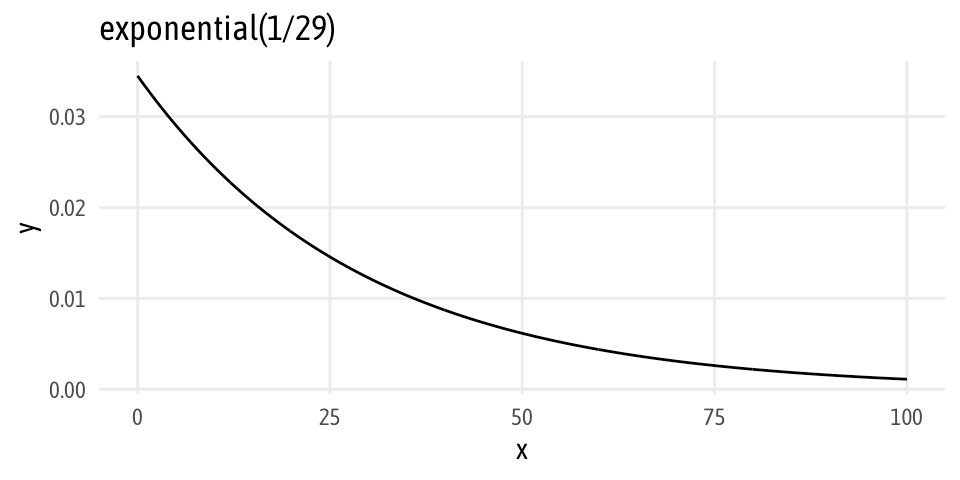
Aí você fala que os graus de liberdade v são distribuídos que nem uma exponential(1/29) (original do Kruschke, 2013)
E manda o brms ou rstan estimar a diferença entre os grupos, média, desvio padrão etc de cada grupo.
Código BRMS
Esse código é para estimar a diferença de média entre os grupos. Nos links lá embaixo tem o código brms caso queira a média também de cada grupo.
troque os argumentos WARMUP e BAYES_SEED de maneira que desejar.
brms_uneq_robust <- brm(
  bf(y ~ x, sigma ~ x),
  family = student,
  data = ...,
  prior = c(set_prior("normal(0, 5)", class = "Intercept"),
            set_prior("normal(0, 1)", class = "b"),
            set_prior("cauchy(0, 1)", class = "b", dpar = "sigma"),
            set_prior("exponential(1.0/29)", class = "nu")),
  chains = CHAINS, iter = ITER, warmup = WARMUP, seed = BAYES_SEED,
  file = "cache/brms_uneq_robust"
)
Código Stan
Esse é mais verboso, mas muito mais poderoso e maleável e estima tanto as médias quanto a diferença.
Além disso já te dá o d de cohen (Cohen, 1988).
// Stan implementation of John Kruschke's Bayesian Estimation Supersedes the
// t-test (BEST), in John K. Kruschke, "Bayesian Estimation Supersedes the t
// test," *Journal of Experimental Psychology* 142, no. 2 (May 2013): 573-603,
// doi:10.1037/a0029146.

// Adapted from code by Michael Clark
// https://github.com/m-clark/Miscellaneous-R-Code/blob/master/ModelFitting/Bayesian/rstant_testBEST.R

// Stuff coming in from R
data {
  int<lower=1> N;  // Sample size
  int<lower=2> n_groups;  // Number of groups
  vector[N] y;  // Outcome variable
  int<lower=1, upper=n_groups> group_id[N];  // Group variable
}

// Stuff to transform in Stan
transformed data {
  real mean_y;
  mean_y = mean(y);
}

// Stuff to estimate
parameters {
  vector[2] mu;  // Estimated group means
  vector<lower=0>[2] sigma;  // Estimated group sd
  real<lower=0, upper=100> nu;  // df for t distribution
}

// Models and distributions
model {
  // Priors
  // curve(expr = dnorm(mean_y, 2), from = -5, to = 5)
  mu ~ normal(mean_y, 2);

  // curve(expr = dcauchy(x, location = 0, scale = 1), from = 0, to = 40)
  sigma ~ cauchy(0, 1);

  // Kruschke uses a nu of exponential(1/29)
  // curve(expr = dexp(x, 1/29), from = 0, to = 200)
  nu ~ exponential(1.0/29);


  // Likelihood
  for (n in 1:N){
    y[n] ~ student_t(nu, mu[group_id[n]], sigma[group_id[n]]);
  }
}

// Stuff to calculate with Stan
generated quantities {
  // Mean difference
  real mu_diff;

  // Effect size; see footnote 1 in Kruschke:2013
  // Standardized difference between two means
  // See https://en.wikipedia.org/wiki/Effect_size#Cohen's_d
  real cohen_d;

  // Common language effect size
  // The probability that a score sampled at random from one distribution will
  // be greater than a score sampled from some other distribution
  // See https://janhove.github.io/reporting/2016/11/16/common-language-effect-sizes
  real cles;

  mu_diff = mu[1] - mu[2];
  cohen_d = mu_diff / sqrt(sum(sigma)/2);
  cles = normal_cdf(mu_diff / sqrt(sum(sigma)), 0, 1);
}
Esses dois artigos falam muito bem aqui:
- Half a dozen frequentist and Bayesian ways to measure the difference in means in two groups | Andrew Heiss
- https://vuorre.netlify.app/post/2017/01/02/how-to-compare-two-groups-with-robust-bayesian-estimation-using-r-stan-and-brms/#robust-bayesian-estimation